
| Previous Page | Experiments Menu | Main Menu | Next Page |
|---|
It is often useful to draw parallels between different fields. The way in which information about an object is transferred by light is very similar to some aspects of radio communication theory and electronics. It turns out that the frequency content of an electrical signal or radio wave is very much like the diffraction pattern of an object.
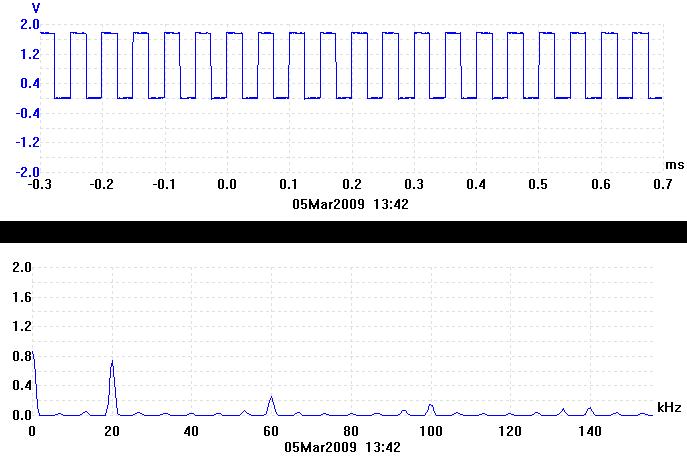
The trace directly below is an oscilloscope trace of a 20kHz voltage square-wave from a signal generator. This is what the square-wave looks like in the time domain. It was captured using a Pico ADC-200 oscilloscope.
The trace directly above is the Fourier transform of the 20kHz square-wave. It represents the frequency spectrum of the square-wave. It is what the square-wave looks like in the frequency domain. Any waveform can be split up into its component sine waves. This is effectively what the Fourier transform does. The Fourier transform of a pure sine wave is just a single peak at the frequency of the sinewave. As can be seen from the trace, the squarewave contains a zero frequency component because it is offset (not centered about 0V). It also contains a 20kHz component which is its fundamental frequency. There are also an infinite number of odd harmonics of the fundamental frequency (60kHz, 100kHz etc.) which add together in the correct way to make up the square-wave.
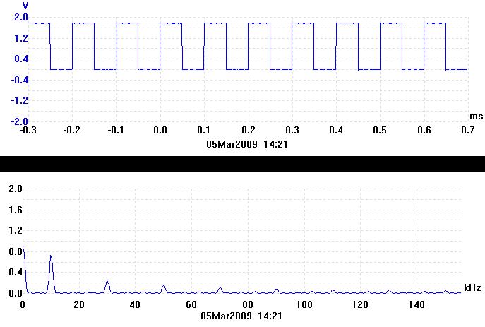
The duration of one cycle of the wave is called the period. The square-wave above has a period of 0.05ms. If the period of the square-wave is doubled, the peaks in the spectrum all get twice as close together. Hence there is a reciprocal relationship between the time domain and the frequency domain. This is illustrated by the next pair of traces. The period has been increased to 0.1ms and the peaks in the frequency domain are now at 10kHz, 30kHz etc.
When the waveform in the time domain is a not a repetitive waveform, its Fourier transform consists of a continuum rather than a series of peaks. The trace below is of a single 0.1ms wide rectangular pulse.
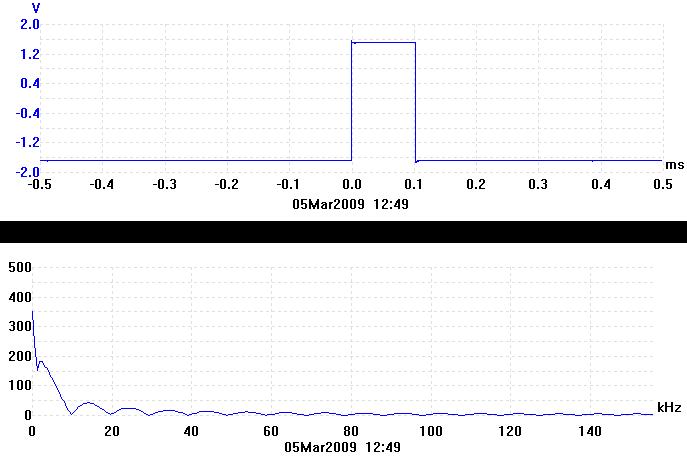
In the frequency domain the rectangular pulse is a continuous curve with minima at 10kHz, 20kHz, 30kHz etc. The shape of this curve is called a sinc2 function. 1 / 0.1ms = 10kHz, which is where the first minima is.
The next trace shows a 0.05ms wide rectangular pulse. It has half the width of the previous pulse.
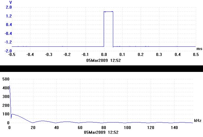
In the frequency domain, the minima have all become twice as far apart, showing the reciprocal relationship again. 1 / 0.05ms = 20kHz, which is where the first minima is.
Finally, the trace below is of a double pulse. The width of each pulse is 0.05ms as before and they are 0.2ms apart.
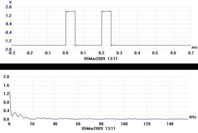
In the frequency domain, the overall envelope of the curve is a sinc2 function with minima at 20kHz, 40kHz etc. as before. Now, however, it is multiplied by a cosine function. The cosine contains the information about how far apart the two rectangular pulses are. 1 / 0.2ms = 5kHz, which is the period of the cosine function in the Fourier transform.
You might be wondering what all this has got to do with the Young's slits experiment. Well, the double pulse shown above represents the pair of slits (object) and the frequency spectrum of that double pulse represents the diffraction pattern produced by the pair of slits. The frequency spectrum of the double pulse, shown above looks very similar to one half of the diffraction pattern produced by Young's double slits. The frequency spectrum of the single pulse is like the diffraction pattern produced by a single slit. Try to remember the shapes of the frequency domain traces for the single and double pulse, you will be seeing them again later.
Fourier transforms work in both directions. Hence, taking the Fourier transform of a Fourier transform gets you back to where you started. A lens performs an optical Fourier transform and hence can turn a diffraction pattern into an image.
The next page describes the construction of the apparatus for the Young's slits experiment.
| Page Title | Description |
|---|---|
| Background | Introduction to diffraction and Young's slits. |
| Project Construction | Information about how the experiment was built. |
| Single Photon Justification | Mathematical justification that the experiment can be considered to be diffracting individual photons. |
| Quiz | A multiple choice quiz (requires Java). |
| Instructions | Instructions for operation of the experiment. |
| Online Experiment | The live interactive Young's slits experiment. Please read the instructions first. |
| Conclusion | Conclusion and references. |
| Previous Page | Experiments Menu | Main Menu | Next Page |
|---|